House Price Analysis using Linear Regression

For a more detailed analysis, check out the full repository on Github. You can even copy the notebook and run the code yourself.

Project Goal

This project is designed to assist a residential real estate company (KC Real Estate) operating in King County. The company primarily helps homeowners sell their homes. The company needs a reliable and efficient way to properly valuate their clients homes. For this to be feasible, they will need a model that can accurately and reliably predict the price of a home given enough data regarding the features of the home.

Using the data provided by the company, I will build regression models in an iterative process to refine my results and create a model that can assist them in setting a preliminary selling price.

Data Preparation

The data for this project is the King County house sales dataset. It contains 21,596 house sales in the county in 2014 and 2015. This project assumes that the data is current, and as a result does not take inflation or other market factors into account.

The dataset can be found here. It is fairly clean already, so it does not require much preparation outside of filling the NaN values and engineering features.

Feature Engineering

Several features included in the dataset are unsuable for a regression analysis, but contain important information, like date. Using the date feature, along with yr_built and yr_renovated, I engineer the following features:

• house_age
• renovated (binary)

Key Metrics and Assumptions

In order to compare the regression models, I will be using the following metrics:

• Root Mean Squared Error (RMSE): measures the standard deviation of the models prediction errors (residuals).
• R-squared: measures goodness-of-fit for the model. The score (ranging between 0-1) will naturally increase as the number of variables in the model increase, so we will also need the adjusted R-squared score.
• Adjusted R-squared: accounts for the number of features included in the model. This score will drop relative to the unadjusted score if the additional features do not improve the model.
• Cross-Validation Score: the mean of the model’s R-squared scores when performed 10 times on different splits of the training data.

I will then validate each model by testing if they meet the assumptions of linear regression. These assumptions are:

• Linearity: the relationship between the independent and dependent variables is linear. As we will see, this assumption no longer applies once we introduce polynomial regression, since our model will no longer be linear.
• Normality: the dependent variable is normally distributed for any fixed value of the independent variables.
• No multi-collinearity: the independent variables are not highly correlated with one another (collinear).
• Homoscedasticity: the variance of the residuals is constant for all values of X.

Regression Models

I begin with a simple linear regression model using only one indepedent variable: sqft_living. This is the independent variable that is most highly correlated with my dependent variable price and has a correlation of 0.702. This model is my baseline that I can compare future models to.

I then build 6 more iterations with varying results. The methods used include:

• increasing the number of independent variables
• normalizing and standardizing the variables
• One-Hot-Encoding the categorical variables
• polynomial regression

Below is a dataframe containing the metrics for each model:

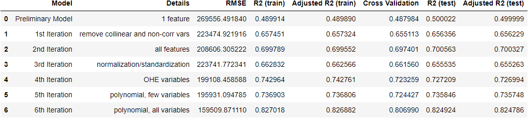
Ultimately, the last model, a polynomial regression model using all variables, was the most accurate. I was performing cursory analysis on each model as I went, but now that I have a final model I will examine and validate it in more detial.

Regression Results and Model Validation

The best model is a 2nd degree polynomial regression model using all variables. The performance metrics are:

• Root Mean Squared Error (RMSE): 159,510
• R-squared (Train): .827
• Adjusted R-squared (Train): .826
• Cross-Validation Score: .807
• R-squared (Test): .825
• Adjusted R-squared (Test): .825

The consistent R-squared scores suggest that the model is not over-fit and can provide consistent results on unseen data. This model significantly outperformed all other models. However, there were some issues when testing the models against the assumptions of linear regression.

• Linearity: the improved performance of the polynomial regression models suggests that the relationship between the independent and dependent variables is not linear. This is not an issue, however, since the final model is not linear either.
• Normality: many of the variables were not normally distributed, so this assumption was not met. Attempting to transform the variables to make them more normal actually negatively affected model performance.
• No Multicollinearity: the most accurate models all had multicollinearity, so this assumption was not met. However, given that the purpose of the model is predictive and not inferential, this is not a major concern. The multiple interactions and collinearity allowed the model to make more accurate predictions, but at the cost of explainability. If the stakeholder had been interested in understanding the relative value each independent variable had when determining price, I would need to focus much more on removing multicollinearity.
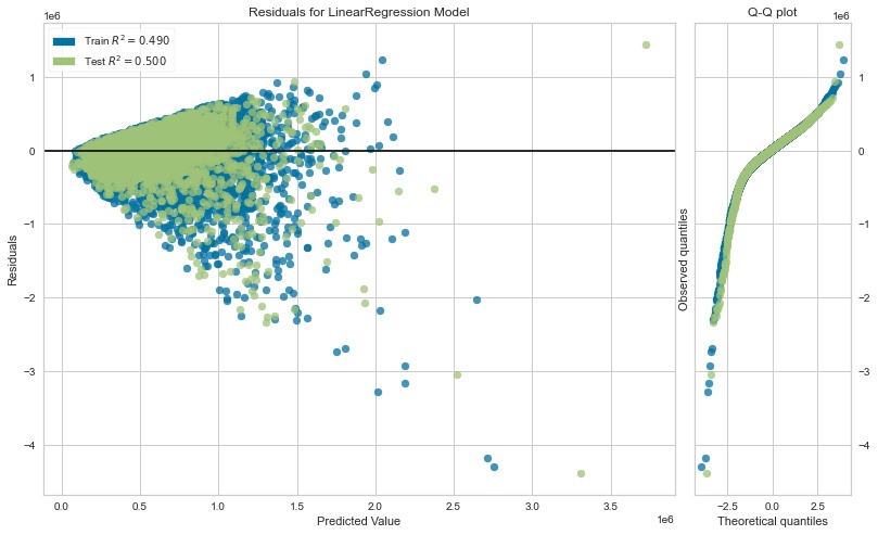
• Homoscedasticity: an initial graphing of the residuals of each model indicated that heteroscedasticity was an issue in most cases, as demonstrated by a cone-shaped residual graph. The graph from the baseline model is shown below:

The least heteroscedastic model, however, was the final model:

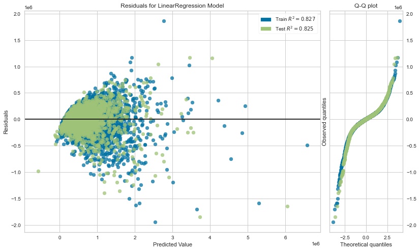
This was a slight surprise, since one of the causes of heteroscedasticity is multicollinearity. I expected the final model to be the most heteroscedastic, but in fact it was the least.

I also examined the model statistics using statsmodels. Here are the results (with the coefficients removed due to the large number of them):

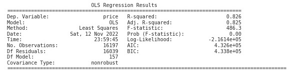
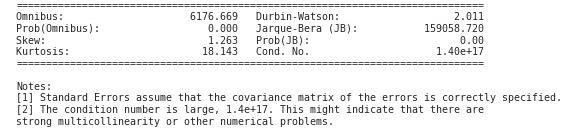
Key takeaways:

• the Omnibus score, as well as the Jarque-Bera score, confirm that the model fails the normality assumption.
• the Durbin-Watson score actually indicates that the model is reasonably homoscedastic, despite the appearance from the residuals graph.
• the Cond. No. confirms that there is high multicollinearity in the model.

Recommendations and Next Steps:

Since the model can only explain 80-82% of the variance of the house price (R-squared), there is still some room for error. The RMSE is 159,510, which means that the standard deviation of the unexplained variance (error) is, on average $159,510. This is fairly large, so the model should not be used without human oversight. The predictions will need to be checked to ensure they make sense given what is known about the home. In particular, because the residuals increase as the actual home price increases, attention should be paid to predictions above a certain threshold. Additionally,

There are several steps that can be taken to try and further improve the model, such as gathering additional data on the homes. It is possible that key features are missing that would increase the accuracy of the model. Additionally, some predictions are negative, so changing the parameters of the model to prevent this could help improve it drastically as well. Alternatively, since the normality and linearity assumptions both failed, it is possible that a method other than regression could provide better insights. It might be worthwhile to consider other types of models that could outperform the current one.