
Statistical Measures in Statsmodels
How to interpret and validate your statistical models

The statsmodels package in python is a very handy tool for evaluating statistical models. It provides an easy way to get a plethora of information on a given model. However, the model summaries can be overwhelming for people who don’t have a background in statistics or mathematics. This article will help you understand the statistical measures that statsmodels provides, allowing you to effectively evaluate your models.
This article assumes a basic understanding of python and some familiarity with statsmodels, but I will provide a brief explanation on how to build a model in statsmodels in order to then evaluate it. The examples I provide are from my project on predicting house prices using linear regression, which can be found at my GitHub repo here.
Building a model in statsmodels
There are multiple ways to build a model in statsmodels, so I will demonstrate one of the most popular and straightforward methods. First, you need to import the library:
import statsmodels.api as sm
Now we need the data. It will need to be stored as 2 separate matrices: one for the dependent variable (y), and one for the indepdenent variables (X). The most common way to store the data is as pandas dataframes, which is what I have done.
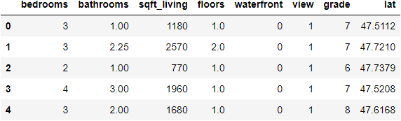
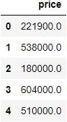
I am using data from the King County house sales dataset, a version of which can be found on Kaggle. I have already cleaned and prepared the data, which includes over 21,000 house sales and over 20 potential variables. I want to create a linear regression model that can predict house prices, so I select several key features (variables) from the dataset that I will use in the model. Here is the first few rows of data that will be used as my independent (X) and dependent (y) variables:
Now that we have the data ready, we can create the model. Normally, you would split your data into training and test sets, but that will be a topic for another post.
If your data does not have a constant, also known as the y-intercept (the ‘b’ in the equation y = mx + b), you need to first create one. It is also important to remember that in statsmodels, the dependent variable is declared before the independent variables. Then fit the data to create the model. Once that is done, we can check the model details by calling model.summary().
# add constant
X = sm.add_constant(X)

# fit data to create model
model = sm.OLS(y, X).fit()

model.summary()
Model Overview
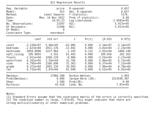
The left side of the top section of the summary includes some basic information about the model that we already know. The Dep. Variable is price, and we are using an OLS (Ordinary Least Squares) linear regression model and method. Also included are the Date and Time that the code was run, the No. Observations, which is the number of data points used, the Df Residuals, which is the degrees of freedom of the model, the Df Model, which is the number of independent variables, and the Covariance Type, which is either robust or nonrobust depending on the methods used to create the model.
On the right side are several important measurements for the model. R-squared and Adj. R-squared measure the amount of variance in the dependent variable that is explained by the independent variables. In this case, the independent variables (X), account for 65.7% of the variance in price. This is not a great score, and indicates that we might be missing some key features that would allow us to predict price more accurately. It is important to compare the R-squared and adjusted R-squared when there is more than one independent variable. Because of the way in which the score is calculated, adding more and more variables will always maintain or inflate the unadjusted score, even if they aren’t useful. The adjusted R-squared score accounts for the number of variables, and the score will drop if the extra variables are not contributing to the model.
The F-statistic is a measurement of statistical significance. It compares the model to a model where all the variable effects are set to 0. The F-statistic then needs to be compared to an F-table using the chosen alpha value to determine if the model is significant. The Prob (F-statistic) provides the probably of the null hypothesis being true, or the chance that the model with all variable effects set to 0 is accurate. In this case, it is at 0, which means that the null hypothesis can be rejected. This does not mean that our model is valid, only that the null hypothesis is invalid.
Log-likelihood, AIC, and BIC are measurements used to compare the coefficient values of the model and influence feature selection.
Coefficients
The middle section of the summary includes detailed information about each independent variable. The variable const is the y-intercept that we added to the model. The constant coefficient is the intercept value when all variables are set to 0. For the other variables, however, the coefficient measures the slope of each variable. That is, the amount of change in price for each unit change of the variable. It is worth noting that if the independent variables have not been standardized, then the units are not equivalent between variables and they should not be used comparatively.
The std err is the standard error of each coefficient, whereas the t value relates to how precisely the coefficient was measured. These two measurements are used to find the t-statistic for each coefficient, which is then used in the column P > |t| to find the p-value. The p-value represents the probability that the coefficient was determined by random chance. The higher the p-value, the greater likelihood that the variable has no actual effect on price, and the results were obtained by chance. This value needs to be compared to the chosen alpha value to be useful, and the alpha value will depend greatly on context and domain. An alpha value of 0.05 is often used, which would mean that if a variable’s p-value exceeds 0.05, then it is likely statistically insignificant and should not be used. However, there is much debate on the efficacy of using p-values to influence feature selection. It is a complicated topic that deserves it’s own post, so for now I will leave it at this.
The next two columns [0.025 0.975] measure the values of the coefficient within 2 standard deviations (95%) of the data, which relates to the previous columns. If a value falls outside of this range, it is often considered to be an outlier.
Model Validation
The bottom section of the summary contains measurements related to the validity of the model. For a linear regression model, this means meeting the four assumptions of linear regression, which are:
- Linearity: the relationship between the independent and dependent variables is linear.
- Normality: the dependent variable is normally distributed for any fixed value of the independent variables.
- No multi-collinearity: the independent variables are not highly correlated with one another (collinear).
- Homoscedasticity: the variance of the residuals is constant for all values of X.
This does not mean that a model that fails to meet all four assumptions is unusable or invalid, but you would want at least some of these assumptions to be met in order to have confidence in the reliability of the model.
The Omnibus and Jarque-Bera scores are alternative methods of determining the normality of the model using skew and kurtosis. A score of 0 indicates perfect normality. The Prob of each score is the probability that the residuals (error) of the model are normally distributed. Our model has very high Omnibus and Jarque-Bera scores, which indicates the data fails the normality assumption. Depending on the situation, this could be something inherent in the data, or something that can be fixed through normalization.
Skew measures the symmetry of the distribution, and Kurtosis measures the height of the distribution’s peak compared to its tails. Perfect skew is indicated by a value of 0, and the Kurtosis value of a normal distribution is 3, with a larger value indicating a steeper peak and more outliers.
The Durbin-Watson score measures the homoscedasticity of the model. The score ranges from 0-4, with a score between 1.5-2.5 generally being considered normal, or homoscedastic, but this is dependent on the context and domain. If the score is outside this range, it indicates possible heteroscedasticity. In our case, the score of 1.993 means that the residuals are likely evenly distributed.
The Cond. No. is the condition number, and as Note [2] at the bottom of the summary indicates, a high condition number likely means there is strong multicollinearity in the model. In the case of our model, we likely have this issue. To solve this, we would need to examine the variables in more detail and try to identify any collinearity or interactions between them, and remove those variables that are causing issues.
Recap
As you can see, there is a lot of information to be gleaned from the statsmodels analysis. Many of these measures and concepts are complex, and would require a great deal more time and attention to cover them fully, so I strongly recommend doing more research into them as necessary. But hopefully, this overview can serve to give you a functional understanding of the statistical information presented, and empower you to better interpret and validate your models in the future.